


Marco C. Goldbarg
Universidade Federal do Rio Grande do Norte
Departamento de Informática e Matemática Aplicada - DIMAp
Professor Titular - Full Professor
The Car Renter Salesman Problem
The Car Renter Salesman Problem (CaRS) is a new variant of the classic Traveling Salesman Problem where the salesman’s tour can be decomposed into contiguous paths that are travelled by different rented cars. The goal is to determine the minimum cost Hamiltonian cycle, considering the cost of the route added to the cost of penalties paid for exchanging vehicles during the route. The penalty is due to fees paid to return the rented cars to their bases.
In general, under the viewpoint of a user of rented cars, the goal is to minimize the costs to move from a starting point to a destination. On the other hand, when someone rents a car, it is assumed that it meets the requirements of comfort and safety. During the travel, in addition to the costs of renting the car, at least the costs of fuel and the payment of fees to travel on the road should be considered. Let G=(N, M, W) be a graph where N={1,...,n} represents the set of vertices, M ={1,...,m} is the set of edges and W={1,...,w} is the set of distances between the vertices or the length of the edges of the set M. The problem described in this paper has the following features:
-
Several types of cars are available for rent, each of them has own characteristics, that is, specific operational costs. These costs include fuel consumption, fees that have to be paid to travel on roads and the value of the rent. The fees that have to be paid to travel on the roads may depend on the type of the car and on the specific roads chosen for the route. The value of the rent can also be associated with a cost per kilometer. Thus, without loss of generality, these costs can be considered as a function of each car on a value associated to the edges (i,j) of graph G. The operational cost of a given car k to traverse an edge (i,j) is denoted by.
-
A car rented in a given company can only be returned in a city where there is an agency of the same company. It is therefore not allowed to rent a car of a given company to travel on a certain segment of the route, if that car cannot be returned on the last city of the segment – there is not an agency of this company in the last city of the segment.
-
Whenever it is possible to rent a car in a city i and return it in city j, i different from j, there is an extra for returning the car to its home city. The variable represents the expense to return car k to city j when it was rented in city i, i different from j.
-
The tour begins and ends in the city where the first car is rented, the city that is the basis for the CaRS.
-
The return cost is null in case the tour is completed with a single car which is delivered in the same town it was rented. This case corresponds to the classic TSP considering the cost of other conditions associated only with the selected car.
-
Cars with the same characteristics rented in a single rental car company can be hired under different costs, depending on the city they where rented or on the contract negotiation. Therefore, without loss of generality, the designation of rent can be efficiently controlled by decisions related to cars, not considering the companies. The set K={1,...,k}, |K|=k is the set of different cars that can be in the solution.
-
The costs of returning the rented car may be strictly associated with the path between the city where the car is delivered and the city where the car was rented or these costs can be a result of independent calculation.
The objective of the proposed problem it to find the hamiltonian cycle that, starting on an initial vertex previously known, minimize the sum of total operating costs of cars in the tour. The total operating costs are composed of a parcel that unifies the rent and other expenses in a value associated to the edges, and a parcel associated to return the car to a city that is not its basis, calculated for each car and for each pair of cities origin/return in the cycle. The CaRS cycle may also be understood as obtained by the union of up to t Hamiltonian paths developed on up to t disjoint subsets of vertices of G. Each of the paths is accomplished with a different car or a car different from those used for the neighboring paths in the cycle. Therefore the cities that compose the cycle can be grouped into up to t different subsets of vertices of G that are covered by cars at least distinct from each other in the neighboring paths in the cycle.
Figure 1 illustrates, in a complete graph with six vertices, a typical instance of CaRS. In the example there are three different rental cars. Figures 1(a), (b) and (c) show the accounting of the costs involved in the displacement of each type of car. Note that, unlike the classical traveling salesman cycle, the solution of CaRS depends on the city chosen to be the starting point of the tour, the basis of the salesman. This fact is due to the rate of return is linked both to the starting city and the direction of devolution. In the example this city is represented by vertex F.
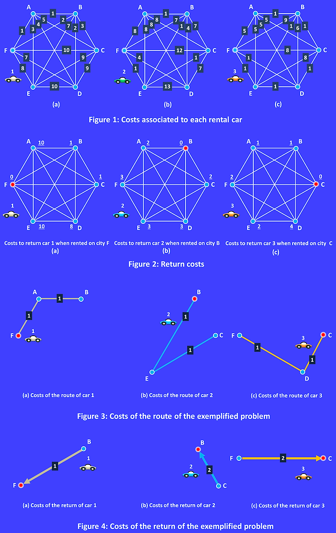
Figure 2 shows, for the example in Figure 1, some of the costs of returning the cars to their bases. Delivery costs appear as underlined numbers next to vertices. Figure 2(a) shows the graph of return of car 1 when rented on vertex F. Figure 2(b) shows the graph of return of car 2 when rented on vertex B and Figure 2(c) the return of car 3 when rented on vertex C. In the general case return costs are known of all cars when rented in any of the cities.
A solution of the problem exemplified in Figures 1 and 2 is exhibited in Figure 3. This solution considers a case where all available cars are rented and no car is rented more than once. The cost of the cycle, according to the solution shown in Figure 3, corresponds to the cost of path F-A-B for car 1, added to the cost of path B-E-C for car 2, added to the cost of path C-D-F of car 3, in a total of 6 unities. To this value it is necessary to add the cost of returning the car to their bases. For car 1, the cost of the return from B to F is one unity. For car 2, the cost of the return from C to B is two unities and, for car 3, the cost to return to C when the car is delivered in F is two unities. Thus, the cost of the final solution is 11 unities.
Figure 4 highlights the return costs of returned cars on the route.